How to show and hide row and column headers in excel

Lori Kaufman
Lori Kaufman
Writer

Lori Kaufman is a technology expert with 25 years of experience. She’s been a senior technical writer, worked as a programmer, and has even run her own multi-location business. Read more.

The headers (numbered rows and lettered columns) in Excel worksheets make it easy to view and reference your data. However, there may be times when the headers are distracting and you don’t want them to display. They are easy to hide and we’ll show you how.

Open the Excel workbook containing the worksheet on which you want to hide the headers. You can activate the worksheet you want by clicking the appropriate tab at the bottom of the Excel window, but you don’t have to. You’ll see why later.

Click the “File” tab.

On the backstage screen, click “Options” in the list of items on the left.

On the “Excel Options” dialog box, click “Advanced” in the list of items on the left.

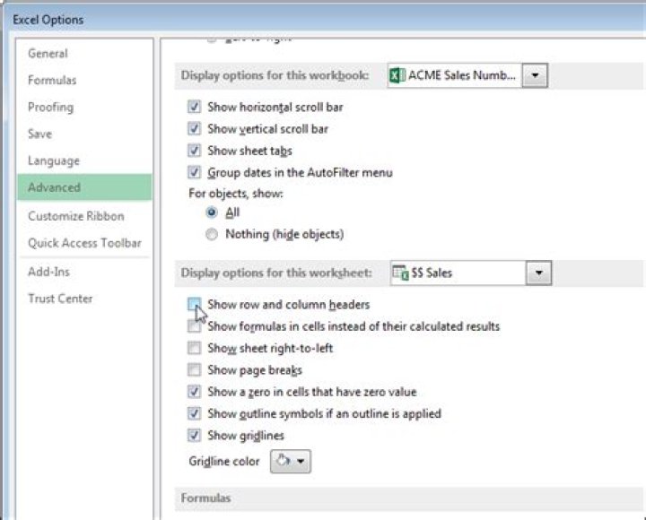
Scroll down to the “Display options for this worksheet” section. If you activated the worksheet for which you want to hide the headers, it’s displayed in the drop-down list on the section heading bar. If not, select the worksheet you want from the drop-down list.

NOTE: All worksheets in all open workbooks display in the drop-down list. You can select a worksheet from any open workbook.

Click the “Show row and column headers” check box so there is NO check mark in the box.

Click “OK” to accept the change and close the “Excel Options” dialog box.

The row and column headers are hidden from view on the selected worksheet. If you activate another worksheet, the row and column headers display again. You can only hide the headers in one worksheet at a time, not all worksheets at once.

Note that Excel does not allow you to show or hide just the row headers or just the column headers. Both the row and columns headers are either displayed or hidden.

• › The Best Gaming Keyboards of 2021: Be on Top of Your Game
• › Why Sublime Text Is Great For Writers, Not Just Programmers
• › What Is a ULED TV, and How Is It Different?
• › Why Professionals Will Actually Want a 2021 MacBook Pro
• › How to Add Images to Questions in Google Forms

Lori Kaufman
Lori Kaufman is a technology expert with 25 years of experience. She’s been a senior technical writer, worked as a programmer, and has even run her own multi-location business.
Read Full Bio »

How to quickly hide unused cells, rows, and columns in Excel?

If you need to keep focus on working in a small part of your worksheet in Excel, you may need to hide the unused cells, rows and columns for achieving it. Here we are going to guide you to hide all unused cells, rows, and columns in Microsoft Excel 2007/2010 quickly.

(4 steps) (1 step)

Hide unused cells, rows, and columns with Hide & Unhide command

We can hide an entire row or column by Hide & Unhide command, and can hide all blank rows and columns with this command too.

Step 1: Select the row header beneath the used working area in the worksheet.

Step 2: Press the shortcut keyboards of Ctrl + Shift + Down Arrow, and then you select all rows beneath the working area.

Step 3: Click the Home > Format > Hide & Unhide > Hide Rows. Then all selected rows beneath working areas are hidden immediately.

Step 4: Same way to hide unused columns: select the column header at the right side of used working area, press the keyboard shortcut of Ctrl + Shift + Right Arrow, and click Home >> Format >> Hide & Unhide >> Hide Columns.

Now all unused cells, rows, and columns are hidden.

Hide unused cells, rows, and columns with Kutools for Excel

If you have Kutools for Excel installed, you can simplify the work and hide unused cells, rows, and columns with only one click.

Kutools for Excel – Includes more than 300 handy tools for Excel. Full feature free trial 30-day, no credit card required! Free Trial Now!

Just select the used working area, and click the Kutools > Show / Hide > Set Scroll Area, then it hides all unused cells, rows, and columns immediately.

Kutools for Excel – Includes more than 300 handy tools for Excel. Full feature free trial 30-day, no credit card required! Get It Now

Demo: hide unused cells, rows, and columns in Excel

One click to hide/unhide one or multiple sheet tabs in Excel

Kutools for Excel provides many handy utilities for Excel users to quickly toggle hidden sheet tabs, hide sheet tabs, or display hidden sheet tabs in Excel. Full Feature Free Trial 30-day!

1. Kutools > Worksheets : One click to toggle all hidden sheet tabs to be visible or invisible in Excel;
2. Kutools > Show / Hide > Hide Unselected Sheets : One click to hide all sheet tabs except active one (or selected ones) in Excel;
3. Kutools > Show / Hide > Unhide All Sheets : One click to display all hidden sheet tabs in Excel.

Kutools for Excel – Includes more than 300 handy tools for Excel. Full feature free trial 30-day, no credit card required! Get It Now

Excel worksheet Row and Column headings are the Column letters at the top of worksheet Columns and Row numbers at the left-side of worksheet Rows.

Excel worksheet Row and Column headings are shown in below image.

The Row numbers and Column letters are one of the fundamental features of Excel worksheet. Row number and Column letter combination is used to identify a Cell in Excel worksheet. The Row numbers and Column Letters make it easy for a user to refer Cells inside Excel worksheet.

Sometimes you may need to hide the Row numbers and Column letters to make more space for worksheet area. You can hide Excel worksheet Row and Column headers or show missing hidden Row and Column headers, by following any of below methods.

Method 1 – Hide/Show Excel worksheet Row and Column headings from Excel Ribbon

To hide Excel worksheet Row and Column headings from Excel Ribbon, follow these steps

Step 1 – Click on "View" Tab on Excel Ribbon.

Step 2 – Go to "Show" Group in Ribbon's "View" Tab.

Step 3 – Uncheck "Headings" checkbox to hide Excel worksheet Row and Column headings.

Check "Headings" checkbox to show missing hidden Excel worksheet Row and Column headings, as explained in below image.

As you can see from the below image, Excel worksheet Gridlines is hidden now.

Method 2 – Hide/Show Excel Row and Column headings from "Excel Options" window

Click the following link if you are not familiar with Excel Options Dialog Box Window

You can achieve the same results explained in above method, using "Excel Options" Window.

Follow below steps to hide Excel Row and Column headings or to show missing hidden Row and Column headings.

Step 1 – Open "Excel Options" window from Excel Backstage View.

Step 2 – Open "Advanced" Panel in "Excel Options" window by clicking on it.

Step 3 – Scroll down to "Display options for this worksheet". Make sure relevant worksheet is selected in "Display options for this worksheet" heading.

Step 4 – Uncheck "Show row and column headers" Checkbox to hide Excel worksheet Row and Column headings

Check "Show row and column headers" Checkbox to show Excel worksheet Row and Column headings, as explained in below image.

Hide or unhide columns in your spreadsheet to show just the data that you need to see or print.

Hide columns

Select one or more columns, and then press Ctrl to select additional columns that aren’t adjacent.

Right-click the selected columns, and then select Hide.

Note: The double line between two columns is an indicator that you’ve hidden a column.

Unhide columns

Select the adjacent columns for the hidden columns.

Right-click the selected columns, and then select Unhide.

Or double-click the double line between the two columns where hidden columns exist.

Do you see double lines at column or row headers instead of the columns or rows, like in this picture?

These double lines mean that some columns and rows are hidden. To see the hidden data, unhide those columns or rows. Whether your data is in a range or a table, here’s how to unhide columns or rows:

Select the columns before and after the hidden columns (like columns C and F in our example).

Right-click the selected column headers and pick Unhide Columns.

Here’s how to unhide rows:

Select the rows before and after the hidden rows (rows 2 and 4 in our example).

Right-click the selected row headers and pick Unhide Rows.

Note: When consecutive columns or rows are hidden, you can’t unhide specific columns or rows. First unhide all the columns or rows, and then hide the ones you don’t want displayed.

Need more help?

You can always ask an expert in the Excel Tech Community or get support in the Answers community.

How to hide row and column headings from all worksheets?

In Excel, we can hide the row and column headings in a worksheet by unchecking the Headings option under the View tab, but, how could you hide the row and column headings from all worksheets in a workbook?

Hide row and column headings from all worksheets with VBA code

Except unchecking the Headings under the View tab one by one, the following VBA code can help you to hide them in all sheets at once.

1. Hold down the ALT + F11 keys to open the Microsoft Visual Basic for Applications window.

2. Click Insert > Module, and paste the following code in the Module Window.

VBA code: Hide row and column headings in all worksheets:

3. Then press F5 key to run this code, and the row and column headings in all worksheets of the active workbook have been hidden at once. See screenshot:

Hide row and column headings from all worksheets with Kutools for Excel

If you have Kutools for Excel, with its View Options feature, you can also hide the row and column headings across all worksheets.

After installing Kutools for Excel, please do as follows:

1. Click Kutools > Show & Hide > View Options, see screenshot:

2. Then in the View Options dialog box, uncheck Row & column headers from the Window options section, and then click Apply to all sheets button, see screenshot:

3. And then the row and column headers in all sheets will be hidden immediately.

When you work on Excel workbook, sometimes, you may need to hide the column and row headers for certain purpose. The powerful tool – Kutools for Excel contains a simple feature can help you to quickly toggle between hiding and showing the column and row headers.

• Reuse Anything: Add the most used or complex formulas, charts and anything else to your favorites, and quickly reuse them in the future.
• More than 20 text features: Extract Number from Text String; Extract or Remove Part of Texts; Convert Numbers and Currencies to English Words.
• Merge Tools : Multiple Workbooks and Sheets into One; Merge Multiple Cells/Rows/Columns Without Losing Data; Merge Duplicate Rows and Sum.
• Split Tools : Split Data into Multiple Sheets Based on Value; One Workbook to Multiple Excel, PDF or CSV Files; One Column to Multiple Columns.
• Paste Skipping Hidden/Filtered Rows; Count And Sum by Background Color ; Send Personalized Emails to Multiple Recipients in Bulk.
• Super Filter: Create advanced filter schemes and apply to any sheets; Sort by week, day, frequency and more; Filter by bold, formulas, comment.
• More than 300 powerful features; Works with Office 2007-2019 and 365; Supports all languages; Easy deploying in your enterprise or organization.

Click Kutools Plus>> Worksheet Design, and a new Design tab will appear in the ribbon, see screenshots:

1. Apply this utility by click Kutools Plus> Worksheet Design, and a Design tab will be displayed in the ribbon, see screenshot:

2. And then check or uncheck the Show Headers option in the View group to toggle showing and hiding column and row headers:

(1.) If you uncheck this Show Headers option, the column and row headers are hidden at once of the current worksheet, see screenshot:

(2.) If you check this option, the column and row headers will be displayed at once, see screenshot:

Note: This feature is only applied to the current worksheet. If you want to show or hide the column and row headers of all worksheets, you can use this View Options function.

Demo: Quickly hide and show column and row headers in current worksheet

Kutools for Excel: with more than 200 handy Excel add-ins, free to try with no limitation in 60 days. Download and free trial Now!

Kutools for Excel

The functionality described above is just one of 300 powerful functions of Kutools for Excel.

Designed for Excel(Office) 2019, 2016, 2013, 2010, 2007 and Office 365. Free download and use for 60 days.

When you create an Excel table, a table Header Row is automatically added as the first row of the table, but you have to option to turn it off or on.

When you first create a table, you have the option of using your own first row of data as a header row by checking the My table has headers option:

If you choose not to use your own headers, Excel will add default header names, like Column1, Column2 and so on, but you can change those at any time. Be aware that if you have a header row in your data, but choose not to use it, Excel will treat that row as data. In the following example, you would need to delete row 2 and rename the default headers, otherwise Excel will mistakenly see it as part of your data.

The screen shots in this article were taken in Excel 2016. If you have a different version your view might be slightly different, but unless otherwise noted, the functionality is the same.

The table header row should not be confused with worksheet column headings or the headers for printed pages. For more information, see Print rows with column headers on top of every page.

When you turn the header row off, AutoFilter is turned off and any applied filters are removed from the table.

When you add a new column when table headers are not displayed, the name of the new table header cannot be determined by a series fill that is based on the value of the table header that is directly adjacent to the left of the new column. This only works when table headers are displayed. Instead, a default table header is added that you can change when you display table headers.

Although it is possible to refer to table headers that are turned off in formulas, you cannot refer to them by selecting them. References in tables to a hidden table header return zero (0) values, but they remain unchanged and return the table header values when the table header is displayed again. All other worksheet references (such as A1 or RC style references) to the table header are adjusted when the table header is turned off and may cause formulas to return unexpected results.

Show or hide the Header Row

Click anywhere in the table.

Go to Table Tools > Design on the Ribbon.

In the Table Style Options group, select the Header Row check box to hide or display the table headers.

If you rename the header rows and then turn off the header row, the original values you input will be retained if you turn the header row back on.

The screen shots in this article were taken in Excel 2016. If you have a different version your view might be slightly different, but unless otherwise noted, the functionality is the same.

The table header row should not be confused with worksheet column headings or the headers for printed pages. For more information, see Print rows with column headers on top of every page.

When you turn the header row off, AutoFilter is turned off and any applied filters are removed from the table.

When you add a new column when table headers are not displayed, the name of the new table header cannot be determined by a series fill that is based on the value of the table header that is directly adjacent to the left of the new column. This only works when table headers are displayed. Instead, a default table header is added that you can change when you display table headers.

Although it is possible to refer to table headers that are turned off in formulas, you cannot refer to them by selecting them. References in tables to a hidden table header return zero (0) values, but they remain unchanged and return the table header values when the table header is displayed again. All other worksheet references (such as A1 or RC style references) to the table header are adjusted when the table header is turned off and may cause formulas to return unexpected results.

Show or hide the Header Row

Click anywhere in the table.

Go to the Table tab on the Ribbon.

In the Table Style Options group, select the Header Row check box to hide or display the table headers.

If you rename the header rows and then turn off the header row, the original values you input will be retained if you turn the header row back on.

Show or hide the Header Row

Click anywhere in the table.

On the Home tab on the ribbon, click the down arrow next to Table and select Toggle Header Row.

Click the Table Design tab > Style Options > Header Row.

Need more help?

You can always ask an expert in the Excel Tech Community or get support in the Answers community.

How to hide/unhide rows or columns with plus or minus sign in Excel?

Normally, we hide or unhide rows and columns by using the Hide or Unhide features from the right-clicking menu. Besides this method, we can hide or unhide rows or columns easily with plus or minus sign in Excel. This article will show you the details.

Hide/unhide rows or columns with plus or minus sign

Please do as follows to hide or unhide rows or columns with plus or minus sign in Excel.

1. Select the entire rows or columns you need to hide or unhide with plus or minus sign, then click Group in the Outline group under Data tab. See screenshot:

2. Then the minus sign is displayed on the left of selected rows, or displayed at the top of the selected columns. Click the minus sign, the selected rows or column are hidden immediately. And click the Plus sign, the hidden rows or columns are showing at once.

Note: For removing the plus or minus sign, please select the rows or columns which you have added plus or minus sign into, then click Ungroup button under Data tab.

Easily hide or unhide range, sheet or window with only one click in Excel:

Kutools for Excel gathers a Show / Hide group as below screenshot shown. With this group, you can easily show or hide ranges, sheets or windows as you need in Excel.
Download the full feature 30-day free trail of Kutools for Excel now!

In this article, we will learn how to show hide Field Header in pivot table in Excel 2016.

For that first, we need to understand how the pivot table works in excel 2016.

A pivot table allows you to extract the data from a large, detailed data set into a customized data set.

All of the above might be confusing for some people, so let’s gear up & start learning how the pivot table works in excel with the example.

Shown below is a data set.

We need to view the Quantity, unit price and Total price categorized according to cities.

We just need to select the data and create its pivot table in just a few simple steps.

Go to Insert > Pivot table

Create Pivot table dialog box appears

Select the Table/Range and choose New worksheet for your new table and click OK.
Your new worksheet will be here like shown below

Now you need to select the fields from the pivot table fields on the right of your sheet.

Now we need Quantity, unit price and Total price categorized according to cities.

Select the required fields to get the pivot table as shown below.

Finally, my data is sorted in a way I wanted.

But I don’t require the field header. To remove the field header. Select Analyze > then unselect field header

You will see that the field header has been removed.

You can create and customize your table with the Pivot table function in Excel.

Hope you understood how to remove field header from the pivot table in Excel 2016. Find more articles on pivot table here. Please share your query below in the comment box. We will assist you.