By Bryan Clark 23 July 2017
When adding information to a spreadsheet, most take the approach of it has to be right the first time, or it’ll involve lots of mundane copy/pasting to fix it later. Excel has dozens of features to help with these sorts of problems if you change your mind later and would like to format your entries in a different way. One of these, Text to Columns, allows you to move text from one column into another, effectively splitting text entries into two separate spaces.
The best use case is for names, but it’ll come in handy for lots of other surprising things the more you use Excel.
1. Open Excel and start a new Blank workbook.
2. Add entries to the first column and select them all.
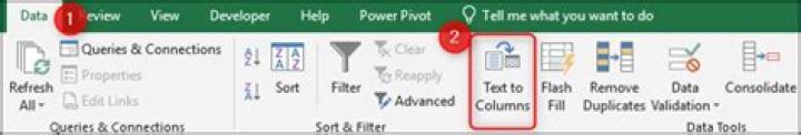
3. Choose the Data tab atop the ribbon.
4. Select Text to Columns.
5. Ensure Delimited is selected and click Next.
6. Clear each box in the Delimiters section and instead choose Comma and Space.
We can use the Text to Column tool to separate values that are not similar into separate columns and rows. This tool helps us to split our data into different columns of the excel sheet. This tutorial will walk all levels of Excel users through the process of Converting Text to Columns and Rows.
Figure 1 – How to Convert Excel Text to Columns and Rows
How to Convert Text to Column
- We will use Figure 2 to illustrate the process of converting text to column.
Figure 2 – Data to convert text to column
- We will select the cells containing our data
Figure 3 – Select the cells with the data
- We will click the Data tab and click Text to columns
Figure 4 – Click Text to Columns
- We will click next
Figure 5 – Convert Text to Columns Wizard
- We will check the Comma and Space boxes
Figure 6 – Check the Comma and Space boxes
- We will click Finish
Figure 7 – Prompt to replace destination cells
- We will click OK
Figure 8 – Text converted to Columns
How to Convert Text to Rows
Excel does not have the Text to Row tool like Text to Column. We will use the Transpose tool to convert our Text to Rows.
- We will select and Copy the data
Figure 9 – How to Convert Text to Rows
- We will select a location where we want our new data to be pasted.
Figure 10 – Select location of new data
- We will right-click and select the Transpose tool under Paste options
Figure 11 – How to convert Text to Rows
Instant Connection to an Expert through our Excelchat Service
Most of the time, the problem you will need to solve will be more complex than a simple application of a formula or function. If you want to save hours of research and frustration, try our live Excelchat service! Our Excel Experts are available 24/7 to answer any Excel question you may have. We guarantee a connection within 30 seconds and a customized solution within 20 minutes.
Text to Columns in Excel (Examples) | How to Convert Text .
› Verified 1 day ago
Start a new line of text inside a cell in Excel – Office .
Excel
› Verified 5 days ago
How to split multiline cell contents into separated rows .
› Verified 1 day ago
Line break as the delimiter in Text to Columns in Excel
› Verified 2 days ago
How to Split Text to Columns in Excel? (Easy and Super Fast)
› Verified 6 days ago
How to Start a NEW LINE in Excel Cell (Windows and Mac)
Excel
› Verified 1 week ago
How to move words to next line in an Excel cell?
› Verified 6 days ago
Using multiple characters as delimiters in Excel Text to .
› Verified 1 week ago
vba – Write each Excel row to new .txt file with ColumnA .
Excel
› Verified 3 days ago
How to split cells in Excel: Text to Columns, Flash Fill .
› Verified 1 week ago
Split Text String by Line Break in Excel – Free Excel Tutorial
› Verified 1 week ago
How to wrap text in Excel automatically and manually
› Verified 4 days ago
Start new line in Excel cell – 3 ways to add carriage return
Excel
› Verified 1 week ago
Resolving text-to-columns with line breaks in Excel
› Verified 1 day ago
Start a new line of text inside a cell in Excel
Excel
› Verified 1 week ago
Text to Columns – Excel – Excel Nerds
› Verified 1 day ago
New Line in Excel Cell | How to Insert or Start a New Line .
Excel
› Verified 1 day ago
How to Add Text to the Beginning or End of all Cells in Excel
› Verified 1 week ago
Start a new line of text inside a cell in Excel – Office .
Excel
› Verified 3 days ago
How to Auto Fill Formula When Inserting New Rows/Data in Excel
› Verified 5 days ago
How to Split Multiple Lines in a Cell into a . – Trump Excel
› Verified 1 day ago
Excel Text Functions – Free Excel Tutorial
› Verified 2 days ago
Drawing a line in Excel | How to Draw line in excel? (with .
Excel
› Verified 1 week ago
Excel Resources – 600+ Self Study Guides, Articles & Tools
Excel
› Verified 4 days ago
Change the column width or row height in Excel – Excel
Excel
› Verified 2 days ago
How to start a new line of text inside a cell in Excel?
Start a new line of text inside a cell in Excel 1 Double-click the cell in which . 2 Click the location inside the . 3 Press Alt+Enter to insert the .
Can you convert text to column in Excel?
You’ve probably had to convert text to columns before in Excel. Usually in one cell, you’ll have a long line of text that is separated by commas, semicolons, or some other delimiter and all you’re trying to do is get each value into its own column. Something along the lines of this:
How to convert text to columns with multiple lines?
Once the text in the cell looks like this, then we are ready to use the Text-to-Columns button to split the text up by the commas that separates each value. The key with using the SUBSTITUTE() function is we want to replace each new line with a comma. The ASCII character code for a new line break is 10 for PCs and 13 for Macs.
How to insert a line break in a cell in Excel?
Press CONTROL+OPTION+RETURN to insert the line break. To start a new line of text or add spacing between lines or paragraphs of text in a worksheet cell, press Alt+Enter to insert a line break. Double-click the cell in which you want to insert a line break (or select the cell and then press F2).
TEXT TO COLUMNS
To separate the contents of one Excel cell into separate columns, you can use the ‘Convert Text to Columns Wizard’. For example, when you want to separate a list of full names into last and first names.
How to splits cells into multiple columns
To use text to a column in excel, please follow below steps:
- Click on home
- Select Range of Cells
- Click on Text to Columns
Result: By clicking on the finish, you will see all the surnames in one column, and the name is another column. This is the process of Text to columns in Excel
We have solved another interesting query of excel users, in case if you wish to convert an invalid date format into a valid date format.
Split Cells into Multiple Columns.
Let’s see how to split the data into multiple columns. This is also part of data cleaning. Sometimes your data are in one single column, and you need to divide it into multiple adjacent columns for applying Sort, Filter or Pivot table.
All the information is in one single column, but you need to separate it. In our earlier example, we have applied the “Delimited” technique. However, this time, we will apply a “Fixed width” strategy of Text to Columns.
Observation:
From the above data, you can understand that there are four pieces of information in a single cell i.e. Account No., Item No., Check No., and Description.
Now you can convert or fix digits with trailing minus into negative digits. Check out how by clicking here:
Our aim is to separate that one column in four different columns. Let’s see how it’s done:
Step 1: Select your data to the range (from the first data cell). Go to the Data tab, and then go to Text to Columns. On the “Convert Text to Columns Wizard – Step 1 of 3” box, choose the Fixed Width option. Click Next.
Step 2: You will see the fixed-width divider vertical line marks (called Break line) in the Data Preview window. You may need to adjust it as per your data structure.
- On double click, the brake line will be deleted
- When you click once, a new brake line will be created at the point of click
- If you click an existing brake line and drag it, it can be moved to the desired position
- After placing appropriate break lines, click Next.
Step 3: As you click on next, you will reach Step 3 of 3 of Text to Columns wizard. You may change the destination cell so that your original data remains intact and output appears in adjoining columns’ cells.
Important Note:
If you click Finish, you will observe that the 3 rd column of the output has last the prefix zeroes i.e. 00816530 gets converted to 816530, thereby corrupting the data.
Step 4: To retain the prefix zeroes, you should have chosen the column from the Data Preview window of Step 3 of 3 of Text to Columns wizard. It will blacken out the column as shown in the picture below.
Step 5: Once the column is blackened out, choose the “Text” option from the list of options [General, Text, Date, and Skip]. Now if you click on Finish, you will see the zeroes are retained in the final output columns.
We have solved another interesting query of quite a few people, in case if you wish to convert an invalid date format into a valid date format. Click here:
How to do text to columns in Excel?
Please find the step below to apply the text to columns in excel
- Click on home
- Select Range of Cells
- Click on Text to Columns
- Choose the Delimited option & Click Next
- Click on the Comma button then the next button.
- Choose Destination cell & Finish
If you like this tutorial, then don’t forget to check our latest Excel Dashboard Course. This course provides excellent quality videos with certification & lifetime access.
Without doubt, an Excel spreadsheet is one of the most advanced tools for working with raw data—and one of the most feared. The application looks complicated, way too advanced, and like something that would take hours to figure out.
I wouldn’t be surprised if upon hearing that you had to start using MS Excel, your heart started to pound. Is there any way to make Microsoft Excel less scary and intimidating? Yes.
By learning a few spreadsheet tricks, you can bring Excel down to your level and start looking at the application in a different light. We rounded up some of the simplest yet powerful MS Excel spreadsheet tips you can start using on your data.
1. Use MS Excel Format Painter
To start you off, get yourself familiar with formatting your spreadsheet cells. A visually organized spreadsheet is highly appreciated by others as it can help them follow your data and calculations easily. To quickly apply your formatting across hundreds of cells, use the Format Painter:
- Select the cell with the formatting you wish to replicate
- Go to the Home menu and click on the Format Painter. Excel will display a paintbrush next to the cursor.
While that paintbrush is visible, click to apply all of the attributes from that cell to any other.
To format a range of cells, double-click the Format Painter during step 1. This will keep the formatting active indefinitely. Use the ESC button to deactivate it when you’re done.
2. Select Entire Spreadsheet Columns or Rows
Another quick tip– use the CTRL and SHIFT buttons to select entire rows and columns.
- Click on the first cell of the data sequence you want to select.
- Hold down CTRL + SHIFT
- Then use the arrow keys to get all the data either above, below or adjacent to the cell you’re in.
You can also use CTRL + SHIFT + * to select your entire data set.
3. Import Data Into Excel Correctly
The benefit of using is Excel is that you can combine different types of data from all kinds of sources. The trick is importing that data properly so you can create Excel drop down lists or pivot tables from it.
Don’t copy-paste complex data sets. Instead, use the options from the Get External Data option under the Data tab. There are specific options for different sources. So use the appropriate option for your data:
4. Enter The Same Data Into Multiple Cells
At one point, you may find yourself needing to enter the same data into a number of different cells. Your natural instinct would be to copy-paste over and over again. But there’s a quicker way:
- Select all the cells where you need the same data filled in (use CTRL + click to select individual cells that are spread across the worksheet)
- In the very last cell you select, type in your data
- Use CTRL+ENTER. The data will be filled in for each cell you selected.
5. Display Excel Spreadsheet Formulas
Jumping into a spreadsheet created by someone else? Don’t worry. You can easily orient yourself and find out which formulas were used. To do this, use the Show Formulas button. Or you can use CTRL + ` on your keyboard. This will give you a view of all formulas used in the workbook.
6. Freeze Excel Rows And Columns
This is a personal favourite of mine when it comes to viewing lengthy spreadsheets. Once you scroll past the first 20 rows, the first row with the column labels annoyingly disappear from view and you begin to lose track of how the data was organized.
To keep them visible, use the Freeze Panes feature under the View menu. You can opt to freeze the top row or, if you have a spreadsheet with numerous columns, you can opt to freeze the first column.
7. Enter Data Patterns Instantly
One great feature in Excel is that it can automatically recognize data patterns. But what’s even better is that Excel will let you enter those data patterns to other cells.
- Simply enter your information in two cells to establish your pattern.
- Highlight the cells. There will be a small square in the bottom right hand corner of the last cell.
- Place your cursor over this square until it becomes a black cross.
- Then click and drag it with your mouse down to populate the cells within a column
8. Hide Spreadsheet Rows and Columns
In some cases, you may have information in rows or columns that are for your eyes only and no one else’s. Isolate these cells from your work area (and prying eyes) by hiding them:
- Select the first column or row in the range you want to hide.
- Go to Format under the Home menu.
- Select Hide & Unhide>Hide Rows or Hide Columns.
To unhide them, click on the first row or column that occur just before and after the hidden range. Repeat steps 2 and 3, but select Unhide Rows or Unhide Columns.
9. Copy Formulas Or Data Between Worksheets
Another helpful tip to know is how to copy formulas and data to a separate worksheet. This is handy when you’re dealing with data that’s spread across different worksheets and requires repetitive calculations.
- With the worksheet containing the formula or data you wish to copy opened, CTRL + click on the tab of the worksheet you want to copy it to.
- Click on or navigate to the cell with the formula or data you need (in the opened worksheet).
- Press F2 to activate the cell.
- Press Enter. This will re-enter the formula or data, and it will also enter it into the same corresponding cell in the other selected worksheet as well.
These general tips won’t turn you into an Excel guru overnight. But they can help you take that first step towards becoming one! Are you a well-seasoned Excel user? Which of your spreadsheet tricks would you add?
By John MacDougall
2019-01-13
DAX | Pivot Tables | Power Pivot
I got a rather interesting question from someone who attended one of my pivot table webinars. They were wondering if they could have text values in the Values area of a pivot table?
This is usually the area where we summarize fields by various different aggregation methods like taking the sum, average, minimum, maximum or standard deviation.
But the thing is, these aggregation methods require numeric data!
Is there any way to summarize text based data that will return text as the result?
The answer is yes, but we will need to use the data model and DAX formulas to do this. Traditional pivot tables do not have this functionality.
Also, we will need to be a PC user with Excel 2013 (or later) and Office 365. Sorry, but these modern features aren’t available in the Mac versions yet.
Table of Contents
Video Tutorial
The Problem
Here we’ve got a list of students along with the courses they are enrolled in. A student can have multiple rows of data when they are enrolled in multiple courses.
Can we summarize this data with a pivot table so that we just display each student once and then show a comma separated list of their courses?
Insert A Pivot Table
First, we will need to insert a pivot table. This is done in the usual manner.
Select a cell inside the data ➜ go to the Insert tab ➜ then press the Pivot Table button.
In order to use DAX formulas, we will need to select the Add this to the Data Model option.
Add A Measure
With traditional pivot tables, we don’t need to define any calculations. They come predefined with basic sum, count, average, minimum, maximum, standard deviation and variance calculations.
With the data model, we get access to a whole new world of possible calculations using DAX formulas. These are created by adding Measures. We can create just about any calculation we can imagine with these.
To add a Measure, select the pivot table ➜ right click on the table of data found in the PivotTable Fields window ➜ choose Add Measure from the menu.
This will open the Measure dialog box where we can create our DAX formulas.
ConcatenateX Function
In the Measure dialog box:
- We need to select the table to which to attach our measure, give the measure a name and description.
- We can explore the available DAX formulas using the Insert Function menu and also check the validity of any formula we write.
- We can write our formula in the DAX formula editor.
- We can assign formatting to the measure.
To create a measure that aggregates text into a comma separated list, we’re going to use the ConcatenateX DAX function.
We need to write the above formula into the DAX formula editor and then we can create the new measure by pressing the OK button.
This will take the Course field from the StudentData table and concatenate its values together with a comma and space character as a delimiter.
Using Our New Measure
This new measure will appear listed in the PivotTable Fields window with all the other fields and we can use this new measure just like any of the other fields.
Measures can easily be identified from the data fields by the fx icon in from of the measure name.
We can click and drag the Course List measure into the Values area of our pivot table and this will produce a comma separated list of a students courses.
Conclusions
Pivot tables have been a feature in Excel for a long time and they can do a lot of great useful calculations.
They are limited though, especially when it comes to displaying text values in the Values area.
With the data model we get many new calculation options that regular pivot tables just don’t have, including concatenating text values to display in the Values area. This is definitely a feature worth exploring when regular pivot tables just won’t cut it.
Wrap text in Excel if you want to display long text on multiple lines in a single cell. Wrap text automatically or enter a manual line break.
Wrap Text Automatically
1. For example, take a look at the long text string in cell A1 below. Cell B1 is empty.
2. On the Home tab, in the Alignment group, click Wrap Text.
3. Click on the right border of the column A header and drag the separator to increase the column width.
4. Double click the bottom border of the row 1 header to automatically adjust the row height.
Note: if you manually set a row height (by clicking on the bottom border of a row header and dragging the separator), Excel does not change the row height when you click the Wrap Text button. Simply double click the bottom border of a row header to fix this.
5. Enter an extra-long text string in cell B1 and wrap the text in this cell.
Note: by default, Excel aligns text to the bottom (see cell A1).
6. Select cell A1.
7. On the Home tab, in the Alignment group, click Top Align.
Manual Line Break
To insert a manual line break, execute the following steps.
1. For example, double click cell A1.
2. Place your cursor at the location where you want the line to break.
3. Press Alt + Enter.
Note: to remove a manual line break, double click a cell, place your cursor at the beginning of the line and press Backspace.
This page is an advertiser-supported excerpt of the book, Power Excel 2010-2013 from MrExcel – 567 Excel Mysteries Solved. If you like this topic, please consider buying the entire e-book.
Problem: I need to type some notes at the bottom of a report. How can I make the words fill each line as if I had typed them in Word?
- This paragraph needs to fit in A:G.
Strategy: You can use Fill, Justify. Follow these steps:
- To have the words fill columns A through G, select a range such as A70:G85. Include enough extra blank rows in the selection to handle the text after word wrapping.
- Select Home, Fill dropdown, Justify. (The Fill dropdown now appears in the Editing group of the Home tab. It often appears as a blue down-arrow icon.)
Results: Excel will rearrange the text to fill each row.
Gotcha: If you have a few words in bold in one cell, this formatting will be lost. Gotcha: If you later change the widths of columns A:G, you will have to use the Justify command again to force the data to fit. Gotcha: Do not use this method if any of your cells contain more than 255 characters. Excel will silently truncate those cells to 255 characters without any notice!
Select Fill Justify.
Alternate Strategy: You can also use a text box to solve this problem. You simply click the Text box icon on the Insert tab, draw a text box to fill columns A through G, and paste your text into the text box. You can then format the text box to hide its border: Select the text box and on the Drawing Tools Format tab, select Shape Outline, None.
Additional Details: Starting in Excel 2007, you can give a text box multiple columns. To do so, you select the text box. On the Drawing Tools Format tab, you click the dialog launcher icon in the bottom-right corner of the Shape Styles group to display the Format Shape dialog. In the left pane, you choose Text Box. Then you click on Columns and specify two columns, with separation between them of 0.1″.
Have you ever split one column in to many columns, or vice versa, combined many columns into a single column? If so, you have likely relied on the text-to-columns feature to split a single column into many and the CONCATENATE function to join many columns into a single column. Beginning with Excel 2013, Microsoft provides an alternative with the introduction of the FlashFill feature. This post explores this feature.
Overview
The quick description of FlashFill is this: it watches you do the first row, and then it extends the pattern down. Now, let’s fill in the details and work through a sample workbook. First up, let’s split a single column into many columns.
Split One Column into Many Columns
In this first example, let’s say that you have a list of transactions with account codes, as shown below.
The account codes were created with three segments, using the following logic:
- XXX is the business unit
- YYYY is the account number
- ZZZ is the department
If we want to generate subtotals by business unit, by account number, or by department, we need to split the account code into the individual segments. Prior to Excel 2013, we could have tackled this task with formulas or with the text-to-columns feature. The text-to-columns feature provides a wizard that allows you to identify the delimiter, in this case a dash, and then Excel would split the values into individual columns. Formulas could also retrieve the individual segments, and common functions used to accomplish this task are LEFT, MID, RIGHT, LEN and FIND. However, we have a new alternative to these approaches beginning with Excel 2013. Let’s use the FlashFill feature here.
All we need to do is enter the first one, and then the FlashFill tries to detect the pattern. It then extends the detected pattern down throughout the range. In this case, we want to pull out the middle segment, the account number segment. So, we simply set up a new column and enter the first one, as shown below.
Then, we just select the first one, and extend our selection through the range, as shown below.
Finally, click the FlashFill button, located in Excel 2013 on the Data ribbon tab. The pattern is extended through the selected range, as shown below.
In my experience, Excel does a good job detecting simple patterns.
Now, let’s go the other way and combine many columns into a single column.
Combine Many Columns into a Single Column
In this example, we have a list of employee names. The names are exported from our HR system with the first name, middle name, and last name columns. We need to combine them into a single column.
The original export is shown below.
We need to combine them, so, we just enter the first one, and then select the whole range, as shown below.
Click the FlashFill button, and Excel attempts to detect the pattern and fill it down, as shown below.
In my experience, this approach is certainly easier and faster than text-to-columns or formulas. For the most part, simple patterns are no problem for FlashFill. However, complex patterns can be a challenge, and when it can’t complete the task, it is good to know we can continue to use our former approaches, text-to-column and formulas.
The file that was used to generate the screenshots is linked below for reference.